Simple Maps with RStudio (UCLA Master's Coursework)

These are some simple, early maps I created with RStudio, rendered in Leaflet.js.

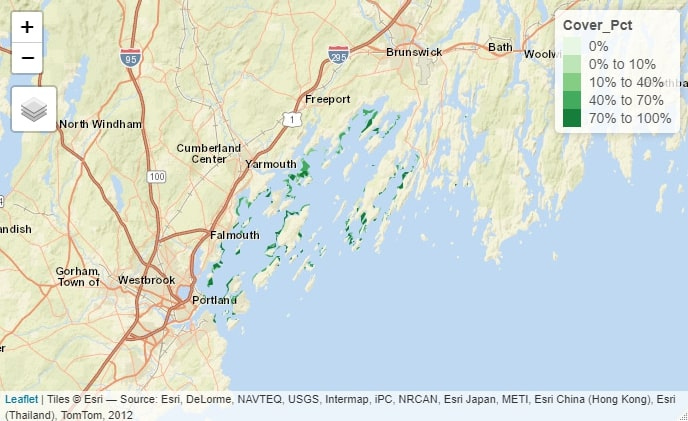
The above map, produced in R's Tmap library, shows eelgrass coverage in Maine’s Casco Bay as of 2018, based on a Maine Department of Environmental Protection dataset and styled with Esri’s World Street Map and a palette of shades of green.

R Code Used:

> eelgrassdata<-st_read("MaineDEP_-_Eelgrass_2018_(Casco_Bay_Only).shp")

>tm_basemap("Esri.WorldStreetMap")+tm_shape(eelgrassdata)+tm_fill("Cover_Pct", palette="Greens")

---

The above map, produced in Tmap, shows major historic, prehistoric, and modern landslides in Maine, based on a Maine Office of GIS dataset and styled with Esri’s World Topo Map and a palette of individually selected colors.

R Code Used:

> landslides<-st_read("Maine_Inland_Landslides_-_Points.shp")

>tm_basemap("Esri.WorldTopoMap")+tm_shape(landslides)+tm_dots("ApproxAge",palette=c(A='cyan', B='red',C='yellow')

---

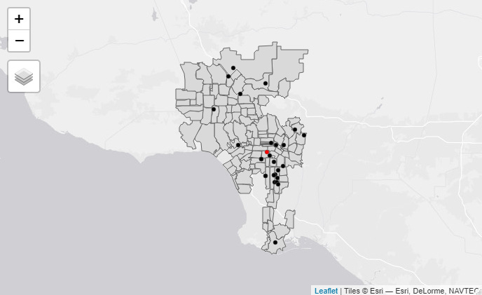
The above map shows criminal homicides in Los Angeles in May 2018. The black points represent homicides, while the red point indicates the spatial mean center of the homicides. Note how the majority of the homicides are concentrated in south and southeast Los Angeles.

R Code used:

> lacrime110<-lacrime[which(lacrime$crimecode==110),]

> tm_shape(lamap)+tm_polygons()+tm_shape(lacrime110)+tm_dots()

> la110xy <- cbind(lacrime110$Longitude, lacrime110$Latitude)

> la110mc<-apply(la110xy,2,mean)

> maplamc110 <- st_sfc(st_point(c(la110mc[1],la110mc[2])))

>tm_shape(lamap)+tm_polygons()+tm_shape(lacrime110)+tm_dots()+tm_shape(maplamc110)+tm_dots(col='red')

The above map calculates the weighted mean center of the US population for each decade and shows how it has moved, on an x-y plane of state centroids.