Georeferencing a 1940s aerial photo (UCLA Master's Coursework)

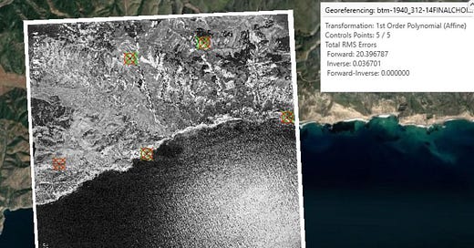
I georeferenced a 1940 black and white aerial photo of part of the coastal area of Santa Cruz Island, California, to the ESRI World Imagery (WGS84) basemap. (The photo source was the UCSB Library FrameFinder archive of historical air photos). The projection is WGS 1984 UTM Zone 11 N. In this "first try" instance, using only a simple first-order polynomial transformation, I created 5 control points (mostly targeting identifiably identical landscape features, like the base of a V-shaped intersection between two cliffs). RMS errors were unfortunately quite high, at 20.396787 forward and 0.036701 inverse.  

In my second step, with a more statistically robust spline transformation, I created 10 control points (again, targeting identifiably identical landscape features). Impressively, Total RMS Errors were reported to be zero, likely due to the increased complexity and accuracy of the spline transformation compared to the first-order polynomial transformation. 

The spline transformation result appears substantially more visually accurate. Using the Swipe tool to view the first-order polynomial transformation reveals several slight “offset” errors, but the spline transformation appears seamless, as can be expected from the difference in total RMS errors. As Esri describes it, the spline transformation uses “a piecewise polynomial that maintains continuity and smoothness between adjacent polynomials” and optimizes for accuracy nearest control points. Here, it appears highly effective